Note
Go to the end to download the full example code
3. Marchenko redatuming with missing sources#
This example shows how the pymarchenko.marchenko.Marchenko
routine can handle acquisition geometries with missing sources. We will first
see that using least-squares inversion leads to retrieving focusing functions
that present gaps due to the missing sources. We further leverage sparsity-
promoting inversion and show that focusing functions can be retrieved that are
almost of the same quality as those constructed with the full acquisition
geometry.
# sphinx_gallery_thumbnail_number = 5
# pylint: disable=C0103
import warnings
import time
import numpy as np
import matplotlib.pyplot as plt

from scipy.signal import convolve
from pylops.basicoperators import Transpose
from pylops.signalprocessing import Radon2D, Sliding2D
from pylops.waveeqprocessing import MDD
from pylops.waveeqprocessing.marchenko import directwave
from pylops.utils.tapers import taper3d
from pymarchenko.marchenko import Marchenko

warnings.filterwarnings('ignore')
plt.close('all')
np.random.seed(10)
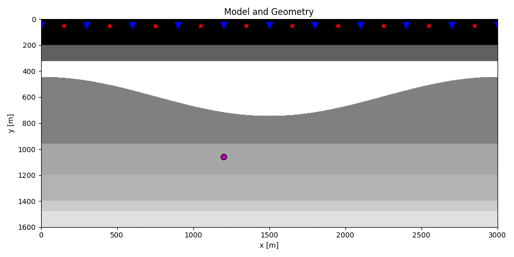
Let’s start by defining some input parameters and loading the geometry
# Input parameters
inputfile = '../testdata/marchenko/input.npz'

vel = 2400.0         # velocity
toff = 0.045         # direct arrival time shift
nsmooth = 10         # time window smoothing
nfmax = 500          # max frequency for MDC (#samples)
nstaper = 11         # source/receiver taper lenght
niter = 10           # iterations

inputdata = np.load(inputfile)

# Receivers
r = inputdata['r']
nr = r.shape[1]
dr = r[0, 1]-r[0, 0]

# Sources
s = inputdata['s']
ns = s.shape[1]
ds = s[0, 1]-s[0, 0]

# Virtual points
vs = inputdata['vs']

# Density model
rho = inputdata['rho']
z, x = inputdata['z'], inputdata['x']

plt.figure(figsize=(10, 5))
plt.imshow(rho, cmap='gray', extent=(x[0], x[-1], z[-1], z[0]))
plt.scatter(s[0, 5::10], s[1, 5::10], marker='*', s=150, c='r', edgecolors='k')
plt.scatter(r[0, ::10], r[1, ::10], marker='v', s=150, c='b', edgecolors='k')
plt.scatter(vs[0], vs[1], marker='.', s=250, c='m', edgecolors='k')
plt.axis('tight')
plt.xlabel('x [m]')
plt.ylabel('y [m]')
plt.title('Model and Geometry')
plt.xlim(x[0], x[-1])
plt.tight_layout()
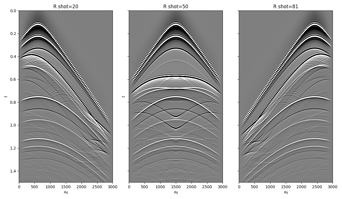
Let’s now load and display the reflection response
# Time axis
t = inputdata['t'][:-100]
ot, dt, nt = t[0], t[1]-t[0], len(t)
t2 = np.concatenate([-t[::-1], t[1:]])
nt2 = 2 * nt - 1

# Reflection data (R[s, r, t]) and subsurface fields
R = inputdata['R'][:, :, :-100]
R = np.swapaxes(R, 0, 1) # just because of how the data was saved
taper = taper3d(nt, [ns, nr], [nstaper, nstaper], tapertype='hanning')
R = R * taper

fig, axs = plt.subplots(1, 3, sharey=True, figsize=(12, 7))
axs[0].imshow(R[20].T, cmap='gray', vmin=-1e-2, vmax=1e-2,
              extent=(r[0, 0], r[0, -1], t[-1], t[0]))
axs[0].set_title('R shot=20')
axs[0].set_xlabel(r'$x_R$')
axs[0].set_ylabel(r'$t$')
axs[0].axis('tight')
axs[0].set_ylim(1.5, 0)
axs[1].imshow(R[ns//2].T, cmap='gray', vmin=-1e-2, vmax=1e-2,
              extent=(r[0, 0], r[0, -1], t[-1], t[0]))
axs[1].set_title('R shot=%d' %(ns//2))
axs[1].set_xlabel(r'$x_R$')
axs[1].set_ylabel(r'$t$')
axs[1].axis('tight')
axs[1].set_ylim(1.5, 0)
axs[2].imshow(R[ns-20].T, cmap='gray', vmin=-1e-2, vmax=1e-2,
              extent=(r[0, 0], r[0, -1], t[-1], t[0]))
axs[2].set_title('R shot=%d' %(ns-20))
axs[2].set_xlabel(r'$x_R$')
axs[2].axis('tight')
axs[2].set_ylim(1.5, 0)
fig.tight_layout()
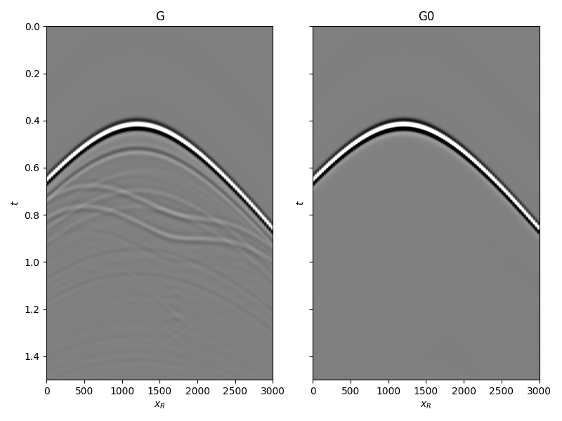
and the true and background subsurface fields
# Subsurface fields
Gsub = inputdata['Gsub'][:-100]
G0sub = inputdata['G0sub'][:-100]
wav = inputdata['wav']
wav_c = np.argmax(wav)

Gsub = np.apply_along_axis(convolve, 0, Gsub, wav, mode='full')
Gsub = Gsub[wav_c:][:nt]
G0sub = np.apply_along_axis(convolve, 0, G0sub, wav, mode='full')
G0sub = G0sub[wav_c:][:nt]

fig, axs = plt.subplots(1, 2, sharey=True, figsize=(8, 6))
axs[0].imshow(Gsub, cmap='gray', vmin=-1e6, vmax=1e6,
              extent=(r[0, 0], r[0, -1], t[-1], t[0]))
axs[0].set_title('G')
axs[0].set_xlabel(r'$x_R$')
axs[0].set_ylabel(r'$t$')
axs[0].axis('tight')
axs[0].set_ylim(1.5, 0)
axs[1].imshow(G0sub, cmap='gray', vmin=-1e6, vmax=1e6,
              extent=(r[0, 0], r[0, -1], t[-1], t[0]))
axs[1].set_title('G0')
axs[1].set_xlabel(r'$x_R$')
axs[1].set_ylabel(r'$t$')
axs[1].axis('tight')
axs[1].set_ylim(1.5, 0)
fig.tight_layout()
First, we use the entire data and create our benchmark solution by means of least-squares inversion
# Direct arrival traveltime
trav = np.sqrt((vs[0]-r[0])**2+(vs[1]-r[1])**2)/vel

MarchenkoWM = Marchenko(R, dt=dt, dr=dr, nfmax=nfmax, wav=wav,
                        toff=toff, nsmooth=nsmooth)

f1_inv_minus, f1_inv_plus, p0_minus, g_inv_minus, g_inv_plus = \
    MarchenkoWM.apply_onepoint(trav, G0=G0sub.T, rtm=True, greens=True,
                               dottest=True, **dict(iter_lim=niter, show=True))
g_inv_tot = g_inv_minus + g_inv_plus
Dot test passed, v^H(Opu)=160.7419881476041 - u^H(Op^Hv)=160.74198814760595
Dot test passed, v^H(Opu)=-159.33392440000824 - u^H(Op^Hv)=-159.33392440000827

LSQR            Least-squares solution of  Ax = b
The matrix A has 282598 rows and 282598 columns
damp = 0.00000000000000e+00   calc_var =        0
atol = 1.00e-06                 conlim = 1.00e+08
btol = 1.00e-06               iter_lim =       10

   Itn      x[0]       r1norm     r2norm   Compatible    LS      Norm A   Cond A
     0  0.00000e+00   2.983e+07  2.983e+07    1.0e+00  3.5e-08
     1  0.00000e+00   1.311e+07  1.311e+07    4.4e-01  9.2e-01   1.1e+00  1.0e+00
     2  0.00000e+00   7.406e+06  7.406e+06    2.5e-01  3.9e-01   1.8e+00  2.2e+00
     3  0.00000e+00   5.479e+06  5.479e+06    1.8e-01  3.3e-01   2.1e+00  3.4e+00
     4  0.00000e+00   3.659e+06  3.659e+06    1.2e-01  3.3e-01   2.5e+00  5.2e+00
     5  0.00000e+00   2.780e+06  2.780e+06    9.3e-02  2.6e-01   2.9e+00  6.8e+00
     6  0.00000e+00   2.244e+06  2.244e+06    7.5e-02  2.3e-01   3.2e+00  8.5e+00
     7  0.00000e+00   1.498e+06  1.498e+06    5.0e-02  2.5e-01   3.6e+00  1.1e+01
     8  0.00000e+00   1.105e+06  1.105e+06    3.7e-02  1.9e-01   3.9e+00  1.3e+01
     9  0.00000e+00   8.988e+05  8.988e+05    3.0e-02  1.6e-01   4.2e+00  1.4e+01
    10  0.00000e+00   6.714e+05  6.714e+05    2.3e-02  1.7e-01   4.4e+00  1.6e+01

LSQR finished
The iteration limit has been reached

istop =       7   r1norm = 6.7e+05   anorm = 4.4e+00   arnorm = 5.1e+05
itn   =      10   r2norm = 6.7e+05   acond = 1.6e+01   xnorm  = 3.5e+07
Second, we define the available sources (60% of the original array randomly selected) and perform least-squares inversion
# Subsampling
perc_subsampling=0.6
nsava = int(np.round(ns*perc_subsampling))
ishuffle = np.random.permutation(np.arange(ns))
iava = np.sort(ishuffle[:nsava])
inotava = np.sort(ishuffle[nsava:])

MarchenkoWM = Marchenko(R[iava], dt=dt, dr=dr, nfmax=nfmax, wav=wav,
                        toff=toff, nsmooth=nsmooth, isava=iava)

f1_inv_minus_ls, f1_inv_plus_ls, p0_minus_ls, g_inv_minus_ls, g_inv_plus_ls = \
    MarchenkoWM.apply_onepoint(trav, G0=G0sub.T, rtm=True,
                               greens=True, dottest=False,
                               **dict(iter_lim=niter, show=True))
g_inv_tot_ls = g_inv_minus_ls + g_inv_plus_ls
LSQR            Least-squares solution of  Ax = b
The matrix A has 170678 rows and 282598 columns
damp = 0.00000000000000e+00   calc_var =        0
atol = 1.00e-06                 conlim = 1.00e+08
btol = 1.00e-06               iter_lim =       10

   Itn      x[0]       r1norm     r2norm   Compatible    LS      Norm A   Cond A
     0  0.00000e+00   2.297e+07  2.297e+07    1.0e+00  4.5e-08
     1  0.00000e+00   7.779e+06  7.779e+06    3.4e-01  1.0e+00   1.1e+00  1.0e+00
     2  0.00000e+00   3.665e+06  3.665e+06    1.6e-01  4.9e-01   1.7e+00  2.1e+00
     3  0.00000e+00   2.263e+06  2.263e+06    9.9e-02  4.2e-01   2.1e+00  3.3e+00
     4  0.00000e+00   1.180e+06  1.180e+06    5.1e-02  3.6e-01   2.4e+00  4.8e+00
     5  0.00000e+00   7.470e+05  7.470e+05    3.3e-02  2.8e-01   2.7e+00  6.1e+00
     6  0.00000e+00   4.771e+05  4.771e+05    2.1e-02  3.0e-01   2.9e+00  7.5e+00
     7  0.00000e+00   3.106e+05  3.106e+05    1.4e-02  2.5e-01   3.2e+00  9.1e+00
     8  0.00000e+00   2.272e+05  2.272e+05    9.9e-03  2.0e-01   3.5e+00  1.1e+01
     9  0.00000e+00   1.663e+05  1.663e+05    7.2e-03  1.8e-01   3.7e+00  1.2e+01
    10  0.00000e+00   1.318e+05  1.318e+05    5.7e-03  1.3e-01   3.9e+00  1.4e+01

LSQR finished
The iteration limit has been reached

istop =       7   r1norm = 1.3e+05   anorm = 3.9e+00   arnorm = 6.5e+04
itn   =      10   r2norm = 1.3e+05   acond = 1.4e+01   xnorm  = 2.4e+07
Finally, we define a sparsifying transform and set up the inversion using
a sparsity promoting solver like pylops.optimization.sparsity.FISTA
# Sliding Radon as sparsifying transform
nwin = 25
nwins = 6
nover = 10
npx = 101
pxmax = 1e-3
px = np.linspace(-pxmax, pxmax, npx)
dimsd = (nr, nt2)
dimss = (nwins*npx, dimsd[1])

Top = Transpose((nt2, nr), axes=(1, 0), dtype=np.float64)
RadOp = Radon2D(t2, np.linspace(-dr*nwin//2, dr*nwin//2, nwin),
                px, centeredh=True, kind='linear', engine='numba')
Slidop = Sliding2D(RadOp, dimss, dimsd, nwin, nover, tapertype='cosine')

MarchenkoWM = Marchenko(R[iava], dt=dt, dr=dr, nfmax=nfmax, wav=wav,
                        toff=toff, nsmooth=nsmooth, isava=iava,
                        S=Top.H*Slidop)

f1_inv_minus_l1, f1_inv_plus_l1, p0_minus_l1, g_inv_minus_l1, g_inv_plus_l1 = \
    MarchenkoWM.apply_onepoint(trav, G0=G0sub.T, rtm=True,
                               greens=True, dottest=False,
                               **dict(eps=1e4, niter=400,
                                      alpha=1.05e-3,
                                      show=True))
g_inv_tot_l1 = g_inv_minus_l1 + g_inv_plus_l1
FISTA (soft thresholding)
--------------------------------------------------------------------------------
The Operator Op has 170678 rows and 1695588 cols
eps = 1.000000e+04      tol = 1.000000e-10      niter = 400
alpha = 1.050000e-03    thresh = 5.250000e+00
--------------------------------------------------------------------------------
   Itn          x[0]              r2norm     r12norm     xupdate
     1       0.0000e+00         2.183e+14   2.189e+14   2.241e+05
     2      -0.0000e+00         1.822e+14   1.833e+14   1.995e+05
     3      -0.0000e+00         1.454e+14   1.471e+14   2.290e+05
     4      -0.0000e+00         1.115e+14   1.137e+14   2.453e+05
     5      -0.0000e+00         8.228e+13   8.517e+13   2.504e+05
     6      -0.0000e+00         5.867e+13   6.216e+13   2.463e+05
     7      -0.0000e+00         4.056e+13   4.463e+13   2.352e+05
     8      -0.0000e+00         2.736e+13   3.197e+13   2.188e+05
     9      -0.0000e+00         1.817e+13   2.328e+13   1.992e+05
    10      -0.0000e+00         1.205e+13   1.762e+13   1.779e+05
    11      -0.0000e+00         8.123e+12   1.410e+13   1.563e+05
    21      -0.0000e+00         6.185e+11   8.215e+12   4.499e+04
    31      -0.0000e+00         1.550e+11   7.391e+12   2.281e+04
    41       0.0000e+00         1.126e+11   6.837e+12   1.849e+04
    51      -0.0000e+00         1.043e+11   6.419e+12   1.747e+04
    61      -0.0000e+00         8.927e+10   6.092e+12   1.738e+04
    71       0.0000e+00         7.796e+10   5.807e+12   1.748e+04
    81       0.0000e+00         7.259e+10   5.554e+12   1.755e+04
    91      -0.0000e+00         7.106e+10   5.329e+12   1.755e+04
   101      -0.0000e+00         6.890e+10   5.130e+12   1.748e+04
   111      -0.0000e+00         6.654e+10   4.954e+12   1.736e+04
   121       0.0000e+00         6.506e+10   4.794e+12   1.723e+04
   131      -0.0000e+00         6.375e+10   4.652e+12   1.702e+04
   141      -0.0000e+00         6.232e+10   4.525e+12   1.679e+04
   151      -0.0000e+00         6.107e+10   4.409e+12   1.655e+04
   161      -0.0000e+00         6.019e+10   4.304e+12   1.628e+04
   171       0.0000e+00         5.945e+10   4.211e+12   1.598e+04
   181      -0.0000e+00         5.898e+10   4.128e+12   1.560e+04
   191      -0.0000e+00         5.831e+10   4.055e+12   1.518e+04
   201      -0.0000e+00         5.764e+10   3.990e+12   1.475e+04
   211       0.0000e+00         5.723e+10   3.932e+12   1.431e+04
   221       0.0000e+00         5.683e+10   3.882e+12   1.383e+04
   231       0.0000e+00         5.639e+10   3.837e+12   1.335e+04
   241       0.0000e+00         5.589e+10   3.797e+12   1.290e+04
   251      -0.0000e+00         5.541e+10   3.763e+12   1.240e+04
   261      -0.0000e+00         5.500e+10   3.731e+12   1.196e+04
   271       0.0000e+00         5.489e+10   3.701e+12   1.157e+04
   281      -0.0000e+00         5.443e+10   3.676e+12   1.114e+04
   291      -0.0000e+00         5.382e+10   3.654e+12   1.071e+04
   301      -0.0000e+00         5.352e+10   3.633e+12   1.035e+04
   311       0.0000e+00         5.324e+10   3.613e+12   1.002e+04
   321      -0.0000e+00         5.302e+10   3.595e+12   9.708e+03
   331      -0.0000e+00         5.290e+10   3.579e+12   9.380e+03
   341      -0.0000e+00         5.268e+10   3.564e+12   9.072e+03
   351       0.0000e+00         5.254e+10   3.551e+12   8.774e+03
   361       0.0000e+00         5.242e+10   3.538e+12   8.524e+03
   371       0.0000e+00         5.225e+10   3.526e+12   8.303e+03
   381      -0.0000e+00         5.187e+10   3.516e+12   8.051e+03
   391      -0.0000e+00         5.174e+10   3.506e+12   7.824e+03
   392      -0.0000e+00         5.173e+10   3.505e+12   7.802e+03
   393      -0.0000e+00         5.172e+10   3.504e+12   7.781e+03
   394      -0.0000e+00         5.172e+10   3.503e+12   7.762e+03
   395      -0.0000e+00         5.171e+10   3.502e+12   7.741e+03
   396      -0.0000e+00         5.170e+10   3.501e+12   7.718e+03
   397      -0.0000e+00         5.168e+10   3.500e+12   7.694e+03
   398      -0.0000e+00         5.167e+10   3.500e+12   7.668e+03
   399      -0.0000e+00         5.165e+10   3.499e+12   7.642e+03
   400      -0.0000e+00         5.164e+10   3.498e+12   7.616e+03

Iterations = 400        Total time (s) = 250.95
--------------------------------------------------------------------------------
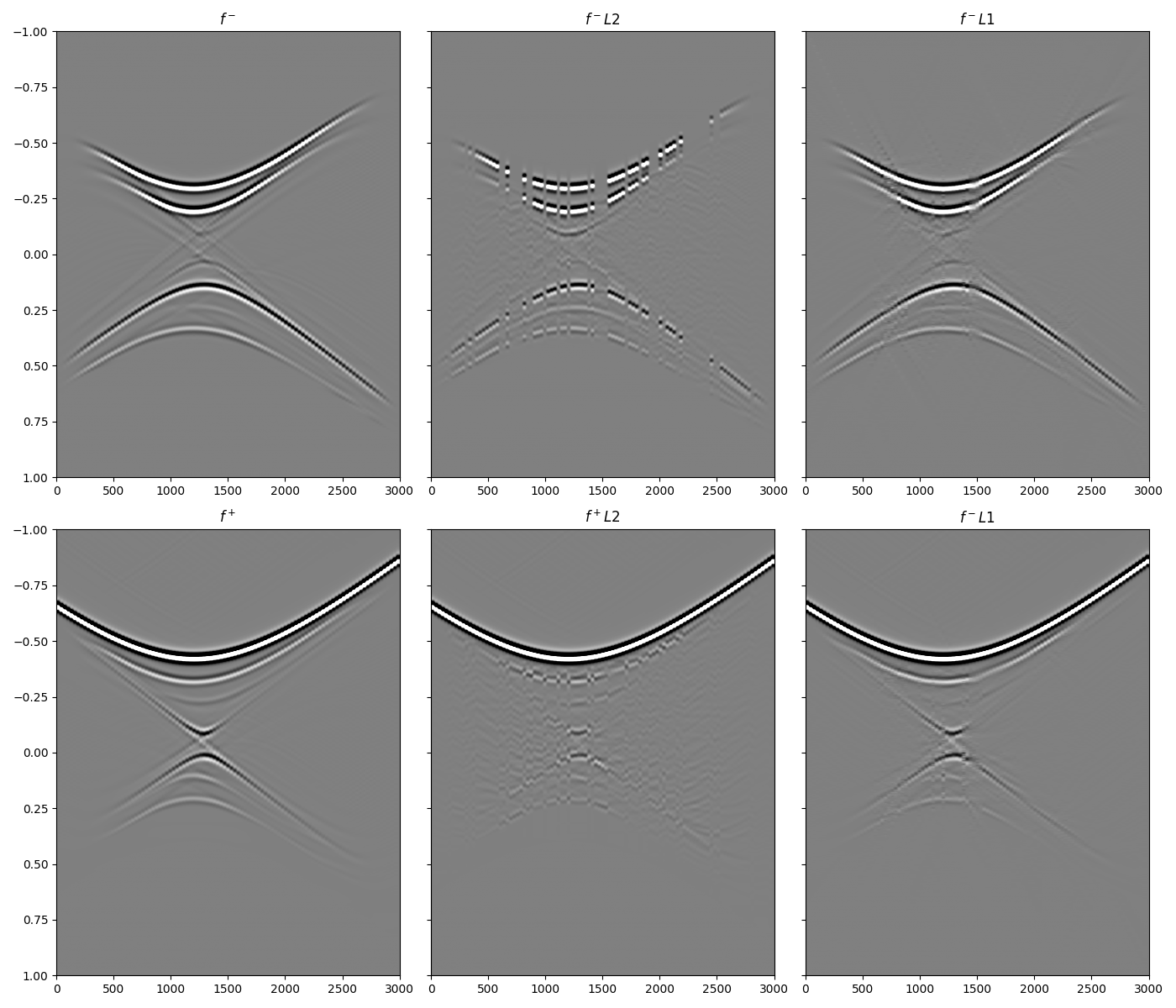
Let’s now compare the three solutions starting from the focusing functions
fig, axs = plt.subplots(2, 3, sharey=True, figsize=(14, 12))
axs[0][0].imshow(f1_inv_minus.T, cmap='gray', vmin=-5e5, vmax=5e5,
                 extent=(r[0, 0], r[0, -1], t2[-1], t2[0]))
axs[0][0].set_title(r'$f^-$')
axs[0][0].axis('tight')
axs[0][0].set_ylim(1, -1)
axs[0][1].imshow(f1_inv_minus_ls.T, cmap='gray', vmin=-5e5, vmax=5e5,
                 extent=(r[0, 0], r[0, -1], t2[-1], t2[0]))
axs[0][1].set_title(r'$f^- L2$')
axs[0][1].axis('tight')
axs[0][1].set_ylim(1, -1)
axs[0][2].imshow(f1_inv_minus_l1.T, cmap='gray', vmin=-5e5, vmax=5e5,
                 extent=(r[0, 0], r[0, -1], t2[-1], t2[0]))
axs[0][2].set_title(r'$f^- L1$')
axs[0][2].axis('tight')
axs[0][2].set_ylim(1, -1)
axs[1][0].imshow(f1_inv_plus.T, cmap='gray', vmin=-5e5, vmax=5e5,
                 extent=(r[0, 0], r[0, -1], t2[-1], t2[0]))
axs[1][0].set_title(r'$f^+$')
axs[1][0].axis('tight')
axs[1][0].set_ylim(1, -1)
axs[1][1].imshow(f1_inv_plus_ls.T, cmap='gray', vmin=-5e5, vmax=5e5,
                 extent=(r[0, 0], r[0, -1], t2[-1], t2[0]))
axs[1][1].set_title(r'$f^+ L2$')
axs[1][1].axis('tight')
axs[1][1].set_ylim(1, -1)
axs[1][2].imshow(f1_inv_plus_l1.T, cmap='gray', vmin=-5e5, vmax=5e5,
                 extent=(r[0, 0], r[0, -1], t2[-1], t2[0]))
axs[1][2].set_title(r'$f^- L1$')
axs[1][2].axis('tight')
axs[1][2].set_ylim(1, -1)
fig.tight_layout()
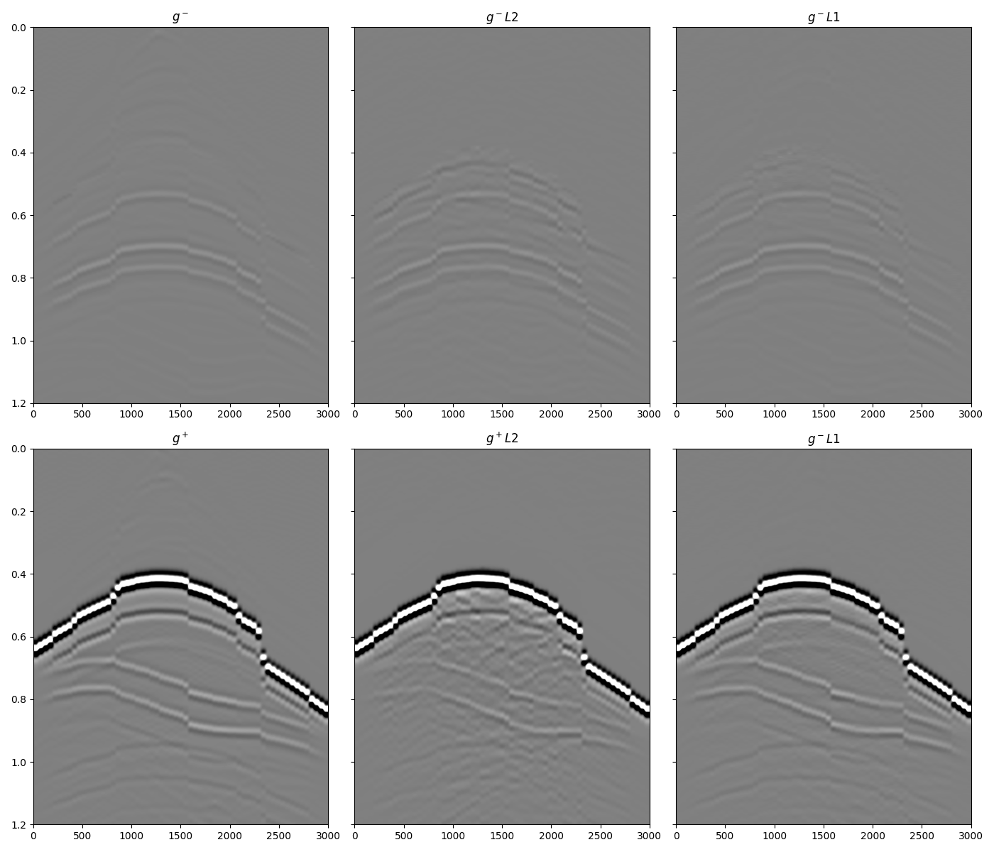
and the up- and down- Green’s functions
fig, axs = plt.subplots(2, 3, sharey=True, figsize=(14, 12))
axs[0][0].imshow(g_inv_minus[iava, :].T, cmap='gray', vmin=-5e5, vmax=5e5,
                 extent=(r[0, 0], r[0, -1], t2[-1], t2[0]))
axs[0][0].set_title(r'$g^-$')
axs[0][0].axis('tight')
axs[0][0].set_ylim(1.2, 0)
axs[0][1].imshow(g_inv_minus_ls.T, cmap='gray', vmin=-5e5, vmax=5e5,
                 extent=(r[0, 0], r[0, -1], t2[-1], t2[0]))
axs[0][1].set_title(r'$g^- L2$')
axs[0][1].axis('tight')
axs[0][1].set_ylim(1.2, 0)
axs[0][2].imshow(g_inv_minus_l1.T, cmap='gray', vmin=-5e5, vmax=5e5,
                 extent=(r[0, 0], r[0, -1], t2[-1], t2[0]))
axs[0][2].set_title(r'$g^- L1$')
axs[0][2].axis('tight')
axs[0][2].set_ylim(1.2, 0)
axs[1][0].imshow(g_inv_plus[iava, :].T, cmap='gray', vmin=-5e5, vmax=5e5,
                 extent=(r[0, 0], r[0, -1], t2[-1], t2[0]))
axs[1][0].set_title(r'$g^+$')
axs[1][0].axis('tight')
axs[1][0].set_ylim(1.2, 0)
axs[1][1].imshow(g_inv_plus_ls.T, cmap='gray', vmin=-5e5, vmax=5e5,
                 extent=(r[0, 0], r[0, -1], t2[-1], t2[0]))
axs[1][1].set_title(r'$g^+ L2$')
axs[1][1].axis('tight')
axs[1][1].set_ylim(1.2, 0)
axs[1][2].imshow(g_inv_plus_l1.T, cmap='gray', vmin=-5e5, vmax=5e5,
                 extent=(r[0, 0], r[0, -1], t2[-1], t2[0]))
axs[1][2].set_title(r'$g^- L1$')
axs[1][2].axis('tight')
axs[1][2].set_ylim(1.2, 0)
fig.tight_layout()
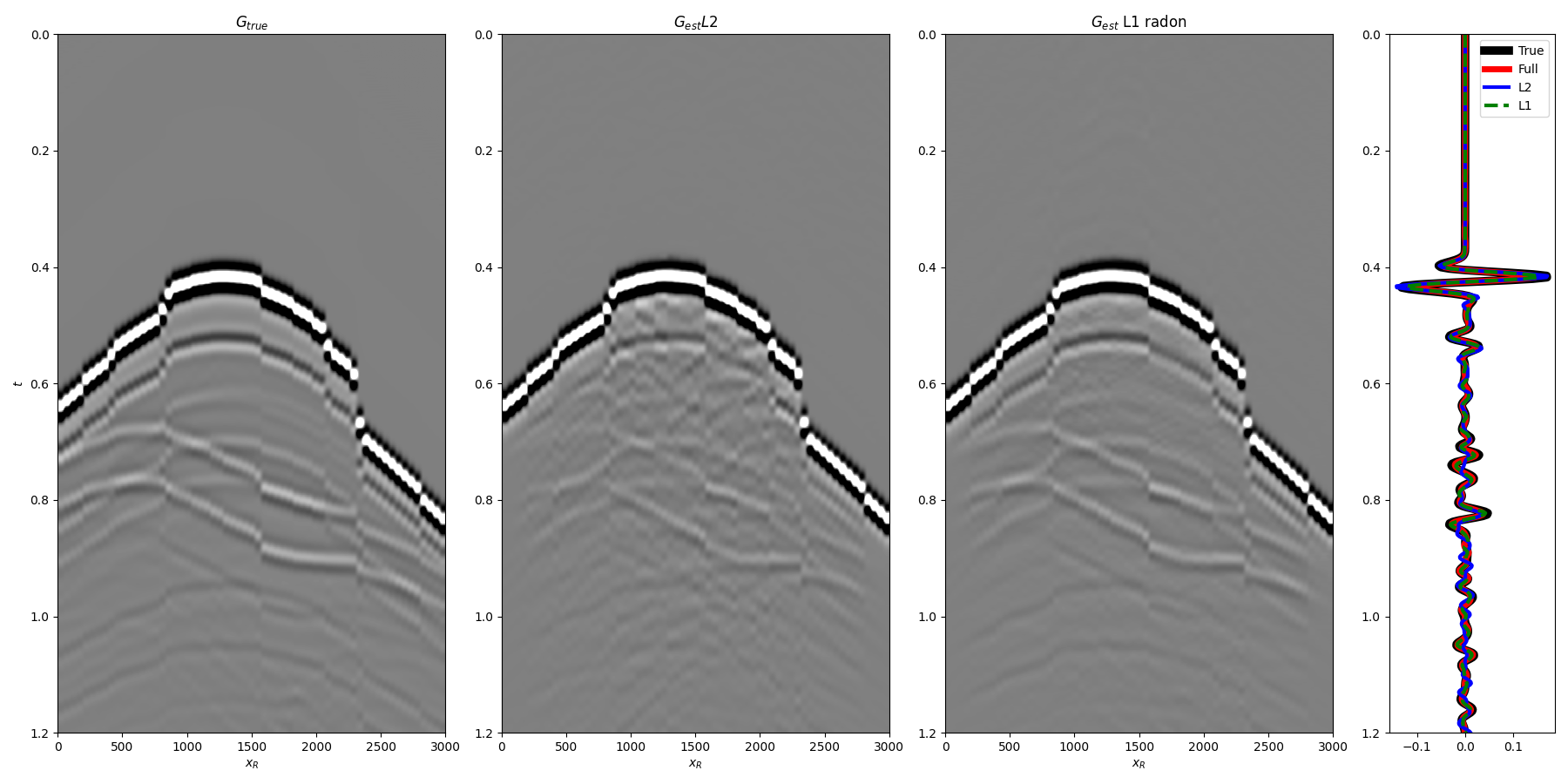
and finally the total Green’s functions
fig = plt.figure(figsize=(18,9))
ax1 = plt.subplot2grid((1, 7), (0, 0), colspan=2)
ax2 = plt.subplot2grid((1, 7), (0, 2), colspan=2)
ax3 = plt.subplot2grid((1, 7), (0, 4), colspan=2)
ax4 = plt.subplot2grid((1, 7), (0, 6))

ax1.imshow(Gsub[:, iava], cmap='gray', vmin=-5e5, vmax=5e5,
           extent=(r[0,0], r[0,-1], t[-1], t[0]))
ax1.set_title(r'$G_{true}$')
ax1.set_xlabel(r'$x_R$')
ax1.set_ylabel(r'$t$')
ax1.axis('tight')
ax1.set_ylim(1.2, 0)
ax2.imshow(g_inv_tot_ls.T, cmap='gray', vmin=-5e5, vmax=5e5,
           extent=(r[0,0], r[0,-1], t2[-1], t2[0]))
ax2.set_title(r'$G_{est} L2$')
ax2.set_xlabel(r'$x_R$')
ax2.axis('tight')
ax2.set_ylim(1.2, 0)
ax3.imshow(g_inv_tot_l1.T, cmap='gray', vmin=-5e5, vmax=5e5,
           extent=(r[0,0], r[0,-1], t2[-1], t2[0]))
ax3.set_title(r'$G_{est}$ L1 radon')
ax3.set_xlabel(r'$x_R$')
ax3.axis('tight')
ax3.set_ylim(1.2, 0)
ax4.plot(t**2*Gsub[:, iava][:, nr//4]/Gsub.max(), t, 'k', lw=7, label='True')
ax4.plot(t**2*g_inv_tot[iava][nr//4, nt-1:]/g_inv_tot.max(), t, 'r', lw=5, label='Full')
ax4.plot(t**2*g_inv_tot_ls[nr//4, nt-1:]/g_inv_tot.max(), t, 'b', lw=3, label='L2')
ax4.plot(t**2*g_inv_tot_l1[nr//4, nt-1:]/g_inv_tot.max(), t, '--g', lw=3, label='L1')
ax4.set_ylim(1.2, 0)
ax4.legend()
fig.tight_layout()
Total running time of the script: (4 minutes 21.084 seconds)