4. Rayleigh-Marchenko redatuming

This example shows how to set-up and run the pymarchenko.raymarchenko.RayleighMarchenko algorithm using synthetic data.

# sphinx_gallery_thumbnail_number = 5
# pylint: disable=C0103
import warnings
import numpy as np

import matplotlib.pyplot as plt

from scipy.signal import convolve
from pymarchenko.raymarchenko import RayleighMarchenko

warnings.filterwarnings('ignore')
plt.close('all')

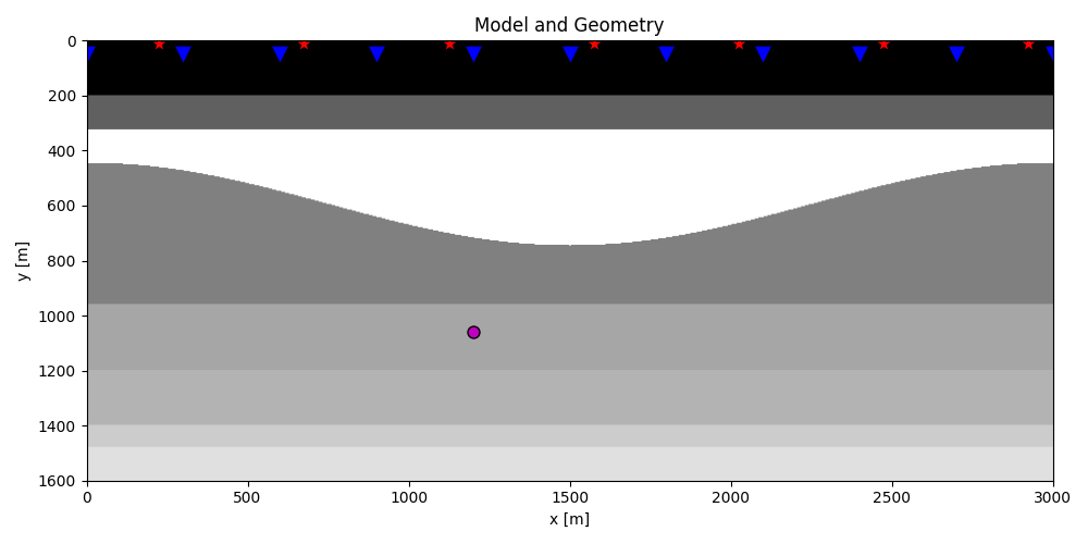
Let’s start by defining some input parameters and loading the geometry

# Input parameters
inputfile = '../testdata/raymarchenko/input.npz'

vel = 2400.0         # velocity
tsoff = 0.06         # direct arrival time shift source side
troff = 0.06         # direct arrival time shift receiver side
nsmooth = 10         # time window smoothing
nfmax = 550          # max frequency for MDC (#samples)
niter = 30           # iterations
convolvedata = True  # Apply convolution to data

inputdata = np.load(inputfile)

# Receivers
r = inputdata['r']
nr = r.shape[1]
dr = r[0, 1]-r[0, 0]

# Sources
s = inputdata['s']
ns = s.shape[1]
ds = s[0, 1]-s[0, 0]

# Virtual points
vs = inputdata['vs']

# Density model
rho = inputdata['rho']
z, x = inputdata['z'], inputdata['x']

plt.figure(figsize=(10, 5))
plt.imshow(rho, cmap='gray', extent=(x[0], x[-1], z[-1], z[0]))
plt.scatter(s[0, 5::10], s[1, 5::10], marker='*', s=150, c='r', edgecolors='k')
plt.scatter(r[0, ::10], r[1, ::10], marker='v', s=150, c='b', edgecolors='k')
plt.scatter(vs[0], vs[1], marker='.', s=250, c='m', edgecolors='k')
plt.axis('tight')
plt.xlabel('x [m]')
plt.ylabel('y [m]')
plt.title('Model and Geometry')
plt.xlim(x[0], x[-1])
plt.tight_layout()

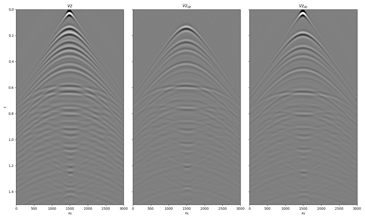
Let’s now load and display the up and downgoing particle velocity data and subsurface fields

# Time axis
t = inputdata['t']
ot, dt, nt = t[0], t[1]-t[0], len(t)

# Wavelet
wav = inputdata['wav']
wav_c = np.argmax(wav)

# Reflection data (R[s, r, t]) and subsurface fields
Vzu = inputdata['Vzu']
Vzd = inputdata['Vzd']

# Convolve data with wavelet
if convolvedata:
    Vzu = dt * np.apply_along_axis(convolve, -1, Vzu, wav, mode='full')
    Vzu = Vzu[..., wav_c:][..., :nt]
    Vzd = dt * np.apply_along_axis(convolve, -1, Vzd, wav, mode='full')
    Vzd = Vzd[..., wav_c:][..., :nt]

fig, axs = plt.subplots(1, 3, sharey=True, figsize=(15, 9))
axs[0].imshow(Vzu[ns//2].T+Vzd[ns//2].T, cmap='gray', vmin=-1e-1, vmax=1e-1,
              extent=(r[0,0], r[0,-1], t[-1], t[0]))
axs[0].set_title(r'$Vz$')
axs[0].set_xlabel(r'$x_R$')
axs[0].set_ylabel(r'$t$')
axs[0].axis('tight')
axs[0].set_ylim(1.5, 0)
axs[1].imshow(Vzu[ns//2].T, cmap='gray', vmin=-1e-1, vmax=1e-1,
              extent=(r[0,0], r[0,-1], t[-1], t[0]))
axs[1].set_title(r'$Vz_{up}$')
axs[1].set_xlabel(r'$x_R$')
axs[1].axis('tight')
axs[1].set_ylim(1.5, 0)
axs[2].imshow(Vzd[ns//2].T, cmap='gray', vmin=-1e-1, vmax=1e-1,
              extent=(r[0,0], r[0,-1], t[-1], t[0]))
axs[2].set_title(r'$Vz_{dn}$')
axs[2].set_xlabel(r'$x_R$')
axs[2].axis('tight')
axs[2].set_ylim(1.5, 0)
fig.tight_layout()

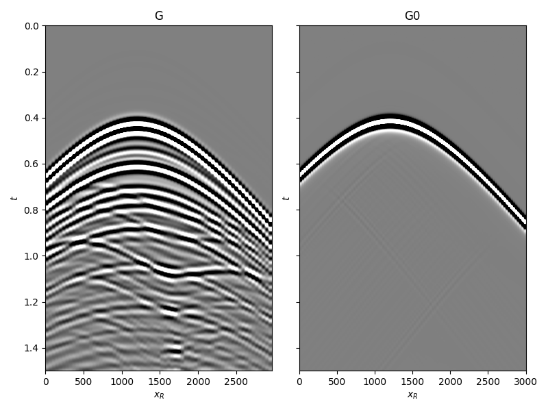
And subsurface fields

Gsub = inputdata['Gsub']
G0sub = inputdata['G0sub']

Gsub = np.apply_along_axis(convolve, 0, Gsub, wav, mode='full')
Gsub = Gsub[wav_c:][:nt]
G0sub = np.apply_along_axis(convolve, 0, G0sub, wav, mode='full')
G0sub = G0sub[wav_c:][:nt]

# Convolve reference Green's function with wavelet
if convolvedata:
    Gsub = dt * np.apply_along_axis(convolve, 0, Gsub, wav, mode='full')
    Gsub = Gsub[wav_c:][:nt]

fig, axs = plt.subplots(1, 2, sharey=True, figsize=(8, 6))
axs[0].imshow(Gsub, cmap='gray', vmin=-1e7, vmax=1e7,
              extent=(s[0, 0], s[0, -1], t[-1], t[0]))
axs[0].set_title('G')
axs[0].set_xlabel(r'$x_R$')
axs[0].set_ylabel(r'$t$')
axs[0].axis('tight')
axs[0].set_ylim(1.5, 0)
axs[1].imshow(G0sub, cmap='gray', vmin=-1e7, vmax=1e7,
              extent=(r[0, 0], r[0, -1], t[-1], t[0]))
axs[1].set_title('G0')
axs[1].set_xlabel(r'$x_R$')
axs[1].set_ylabel(r'$t$')
axs[1].axis('tight')
axs[1].set_ylim(1.5, 0)
fig.tight_layout()

Let’s now create an object of the pymarchenko.raymarchenko.RayleighMarchenko class and apply redatuming for a single subsurface point vs.

# Direct arrival traveltimes
travs = np.sqrt((vs[0]-s[0])**2+(vs[1]-s[1])**2)/vel
travr = np.sqrt((vs[0]-r[0])**2+(vs[1]-r[1])**2)/vel

rm = RayleighMarchenko(Vzd, Vzu, dt=dt, dr=dr,
                       nfmax=nfmax, wav=wav, toff=troff, nsmooth=nsmooth,
                       dtype='float64', saveVt=True, prescaled=False)

f1_inv_minus, f1_inv_plus, p0_minus, g_inv_minus, g_inv_plus = \
    rm.apply_onepoint(travs, travr, G0=G0sub.T, rtm=True, greens=True,
                      dottest=True, **dict(iter_lim=niter, show=True))
g_inv_tot = -(g_inv_minus + g_inv_plus)

Dot test passed, v^H(Opu)=-62.2757380961439 - u^H(Op^Hv)=-62.2757380961445
Dot test passed, v^H(Opu)=-26.251245996755546 - u^H(Op^Hv)=-26.25124599675556

LSQR            Least-squares solution of  Ax = b
The matrix A has 267866 rows and 403798 columns
damp = 0.00000000000000e+00   calc_var =        0
atol = 1.00e-06                 conlim = 1.00e+08
btol = 1.00e-06               iter_lim =       30

   Itn      x[0]       r1norm     r2norm   Compatible    LS      Norm A   Cond A
     0  0.00000e+00   7.383e+08  7.383e+08    1.0e+00  9.4e-10
     1  9.04919e+04   5.220e+08  5.220e+08    7.1e-01  6.3e-01   9.9e-01  1.0e+00
     2  2.20830e+04   3.413e+08  3.413e+08    4.6e-01  4.4e-01   1.4e+00  2.5e+00
     3  8.57234e+04   2.912e+08  2.912e+08    3.9e-01  3.7e-01   1.9e+00  4.0e+00
     4  1.91895e+05   2.297e+08  2.297e+08    3.1e-01  2.4e-01   2.6e+00  6.3e+00
     5  1.99985e+05   1.924e+08  1.924e+08    2.6e-01  1.9e-01   2.9e+00  8.1e+00
     6  2.28755e+05   1.683e+08  1.683e+08    2.3e-01  1.3e-01   3.2e+00  9.9e+00
     7  4.20123e+05   1.461e+08  1.461e+08    2.0e-01  1.5e-01   3.4e+00  1.2e+01
     8  4.20946e+05   1.258e+08  1.258e+08    1.7e-01  1.3e-01   3.7e+00  1.4e+01
     9  4.32414e+05   1.122e+08  1.122e+08    1.5e-01  1.1e-01   3.9e+00  1.7e+01
    10  5.42342e+05   1.019e+08  1.019e+08    1.4e-01  1.0e-01   4.1e+00  1.9e+01
    20  5.75490e+05   4.917e+07  4.917e+07    6.7e-02  5.5e-02   5.8e+00  4.9e+01
    21  5.41632e+05   4.596e+07  4.596e+07    6.2e-02  5.3e-02   6.0e+00  5.3e+01
    22  5.01525e+05   4.297e+07  4.297e+07    5.8e-02  4.9e-02   6.1e+00  5.6e+01
    23  4.61134e+05   4.019e+07  4.019e+07    5.4e-02  4.8e-02   6.2e+00  6.0e+01
    24  4.38557e+05   3.813e+07  3.813e+07    5.2e-02  4.4e-02   6.3e+00  6.3e+01
    25  4.04307e+05   3.613e+07  3.613e+07    4.9e-02  4.3e-02   6.4e+00  6.7e+01
    26  3.47775e+05   3.398e+07  3.398e+07    4.6e-02  4.5e-02   6.5e+00  7.1e+01
    27  3.29531e+05   3.203e+07  3.203e+07    4.3e-02  4.0e-02   6.6e+00  7.5e+01
    28  3.30142e+05   3.029e+07  3.029e+07    4.1e-02  4.0e-02   6.7e+00  7.8e+01
    29  3.26705e+05   2.887e+07  2.887e+07    3.9e-02  4.0e-02   6.8e+00  8.2e+01
    30  3.27919e+05   2.741e+07  2.741e+07    3.7e-02  3.6e-02   6.9e+00  8.6e+01

LSQR finished
The iteration limit has been reached

istop =       7   r1norm = 2.7e+07   anorm = 6.9e+00   arnorm = 6.8e+06
itn   =      30   r2norm = 2.7e+07   acond = 8.6e+01   xnorm  = 1.8e+09

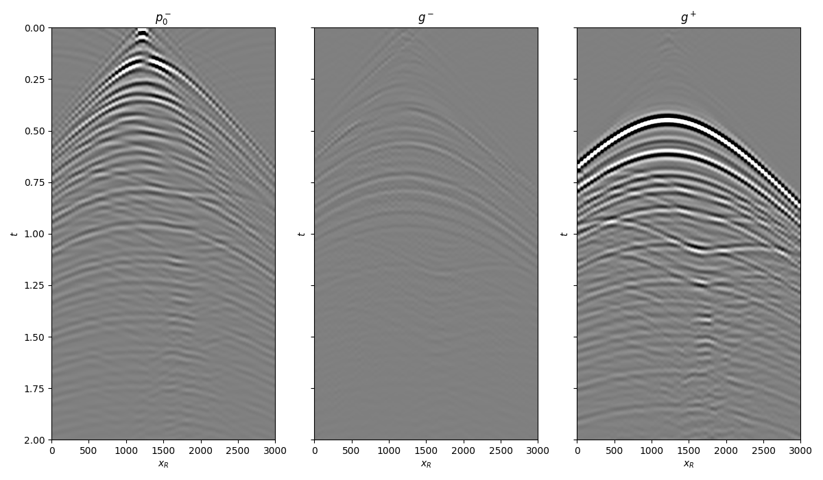
We can now compare the result of Rayleigh-Marchenko redatuming with standard redatuming

fig, axs = plt.subplots(1, 3, sharey=True, figsize=(12, 7))
axs[0].imshow(p0_minus.T, cmap='gray', vmin=-1e7, vmax=1e7,
              extent=(r[0, 0], r[0, -1], t[-1], -t[-1]))
axs[0].set_title(r'$p_0^-$')
axs[0].set_xlabel(r'$x_R$')
axs[0].set_ylabel(r'$t$')
axs[0].axis('tight')
axs[0].set_ylim(2, 0)
axs[1].imshow(g_inv_minus.T, cmap='gray', vmin=-1e7, vmax=1e7,
              extent=(r[0, 0], r[0, -1], t[-1], -t[-1]))
axs[1].set_title(r'$g^-$')
axs[1].set_xlabel(r'$x_R$')
axs[1].set_ylabel(r'$t$')
axs[1].axis('tight')
axs[1].set_ylim(2, 0)
axs[2].imshow(g_inv_plus.T, cmap='gray', vmin=-1e7, vmax=1e7,
              extent=(r[0, 0], r[0, -1], t[-1], -t[-1]))
axs[2].set_title(r'$g^+$')
axs[2].set_xlabel(r'$x_R$')
axs[2].set_ylabel(r'$t$')
axs[2].axis('tight')
axs[2].set_ylim(2, 0)
fig.tight_layout()

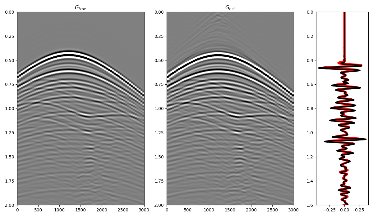
And compare the total Green’s function with the directly modelled one

fig = plt.figure(figsize=(12, 7))
ax1 = plt.subplot2grid((1, 5), (0, 0), colspan=2)
ax2 = plt.subplot2grid((1, 5), (0, 2), colspan=2)
ax3 = plt.subplot2grid((1, 5), (0, 4))
ax1.imshow(Gsub / Gsub.max(), cmap='gray', vmin=-3e-1, vmax=3e-1,
           extent=(r[0, 0], r[0, -1], t[-1], t[0]))
ax1.set_title(r'$G_{true}$')
axs[0].set_xlabel(r'$x_R$')
axs[0].set_ylabel(r'$t$')
ax1.axis('tight')
ax1.set_ylim(2, 0)
ax2.imshow(g_inv_tot.T / g_inv_tot.max(), cmap='gray', vmin=-3e-1, vmax=3e-1,
           extent=(r[0, 0], r[0, -1], t[-1], -t[-1]))
ax2.set_title(r'$G_{est}$')
axs[1].set_xlabel(r'$x_R$')
axs[1].set_ylabel(r'$t$')
ax2.axis('tight')
ax2.set_ylim(2, 0)
ax3.plot(Gsub[:, ns//2] / Gsub.max() * (t ** 1.5), t, 'r', lw=5)
ax3.plot(g_inv_tot[ns//2, nt-1:] / g_inv_tot.max() * (t ** 1.5), t, 'k', lw=3)
ax3.set_ylim(1.6, 0)
fig.tight_layout()