5. Marchenko Multiple Elimination

This example performs internal multiple elimination using the pymarchenko.mme.MME routine. The MME algorithm can also compensate for transmission losses provided a proper choice of the windowing function, here we show how this can be done with our routine.

In this tutorial, we will demultiple only a small portion of the data. Consult the notebooks in the repository for a complete example.

# sphinx_gallery_thumbnail_number = 3
# pylint: disable=C0103
import warnings
import os
import numpy as np
import matplotlib.pyplot as plt

from scipy.signal import convolve
from pymarchenko.mme import MME

warnings.filterwarnings('ignore')
plt.close('all')

os.environ["OMP_NUM_THREADS"] = "1"
os.environ["MKL_NUM_THREADS"] = "1"

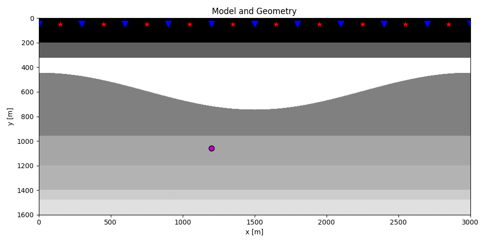
Let’s start by defining some input parameters and loading the geometry

# Input parameters
inputfile = '../testdata/marchenko/input.npz'

vel = 2400.0         # velocity
toff = 0.045         # direct arrival time shift
nsmooth = 10         # time window smoothing
nfmax = 400          # max frequency for MDC (#samples)
niter = 10           # iterations
ntmax = 200          # maximum time of data to demultiple

inputdata = np.load(inputfile)

# Receivers
r = inputdata['r']
nr = r.shape[1]
dr = r[0, 1]-r[0, 0]

# Sources
s = inputdata['s']
ns = s.shape[1]
ds = s[0, 1]-s[0, 0]

# Virtual points
vs = inputdata['vs']

# Density model
rho = inputdata['rho']
z, x = inputdata['z'], inputdata['x']

plt.figure(figsize=(10, 5))
plt.imshow(rho, cmap='gray', extent=(x[0], x[-1], z[-1], z[0]))
plt.scatter(s[0, 5::10], s[1, 5::10], marker='*', s=150, c='r', edgecolors='k')
plt.scatter(r[0, ::10], r[1, ::10], marker='v', s=150, c='b', edgecolors='k')
plt.scatter(vs[0], vs[1], marker='.', s=250, c='m', edgecolors='k')
plt.axis('tight')
plt.xlabel('x [m]')
plt.ylabel('y [m]')
plt.title('Model and Geometry')
plt.xlim(x[0], x[-1])
plt.tight_layout()

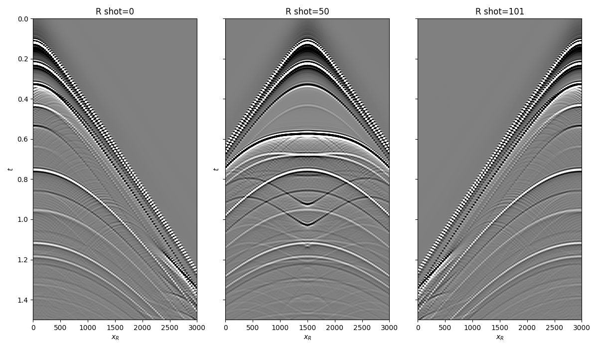
Let’s now load and display the reflection response

# Time axis
t = inputdata['t'][:-100]
ot, dt, nt = t[0], t[1]-t[0], len(t)

# Reflection data (R[s, r, t])
R = inputdata['R'][:, :, :-100]
R = np.swapaxes(R, 0, 1) # just because of how the data was saved
wav = inputdata['wav']
wav_c = np.argmax(wav)

fig, axs = plt.subplots(1, 3, sharey=True, figsize=(12, 7))
axs[0].imshow(R[0].T, cmap='gray', vmin=-1e-2, vmax=1e-2,
              extent=(r[0, 0], r[0, -1], t[-1], t[0]))
axs[0].set_title('R shot=0')
axs[0].set_xlabel(r'$x_R$')
axs[0].set_ylabel(r'$t$')
axs[0].axis('tight')
axs[0].set_ylim(1.5, 0)
axs[1].imshow(R[ns//2].T, cmap='gray', vmin=-1e-2, vmax=1e-2,
              extent=(r[0, 0], r[0, -1], t[-1], t[0]))
axs[1].set_title('R shot=%d' %(ns//2))
axs[1].set_xlabel(r'$x_R$')
axs[1].set_ylabel(r'$t$')
axs[1].axis('tight')
axs[1].set_ylim(1.5, 0)
axs[2].imshow(R[-1].T, cmap='gray', vmin=-1e-2, vmax=1e-2,
              extent=(r[0, 0], r[0, -1], t[-1], t[0]))
axs[2].set_title('R shot=%d' %ns)
axs[2].set_xlabel(r'$x_R$')
axs[2].axis('tight')
axs[2].set_ylim(1.5, 0)
fig.tight_layout()

Let’s now create an object of the pylops.mme.MME class and apply multiple elimination for a single source.

Rwav = R[ns//2].T
Rwav = np.apply_along_axis(convolve, 0, Rwav, wav, mode='full')
Rwav = Rwav[wav_c:][:nt]

MarchenkoMME = MME(R, wav, wav_c, nt=nt, dt=dt, dr=dr,
                   toff=toff, nsmooth=nsmooth)

U_minus = MarchenkoMME.apply_onesrc(R[ns//2], ntmax=ntmax, n_iter=niter)

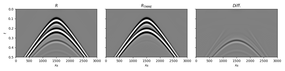
We can now compare the original dataset with the demultipled one

fig, axs = plt.subplots(1, 3, sharey=True, figsize=(12, 3))
axs[0].imshow(Rwav[:ntmax], cmap='gray', vmin=-1e-1, vmax=1e-1,
              extent=(r[0, 0], r[0, -1], t[ntmax], t[0]))
axs[0].set_title(r'$R$')
axs[0].set_xlabel(r'$x_R$')
axs[0].set_ylabel(r'$t$')
axs[0].axis('tight')
axs[1].imshow(U_minus[:, :ntmax].T, cmap='gray', vmin=-1e-1, vmax=1e-1,
              extent=(r[0, 0], r[0, -1], t[ntmax], t[0]))
axs[1].set_title(r'$R_{TMME}$')
axs[1].set_xlabel(r'$x_R$')
axs[1].axis('tight')
axs[2].imshow(Rwav[:ntmax] - U_minus[:, :ntmax].T,
              cmap='gray', vmin=-1e-1, vmax=1e-1,
              extent=(r[0, 0], r[0, -1], t[ntmax], t[0]))
axs[2].set_title(r'$Diff.$')
axs[2].set_xlabel(r'$x_R$')
axs[2].axis('tight')
fig.tight_layout()