1. Marchenko redatuming by iterative substitution

This example shows how to set-up and run the pymarchenko.neumarchenko.NeumannMarchenko algorithm using synthetic data.

# sphinx_gallery_thumbnail_number = 5
# pylint: disable=C0103
import warnings
import numpy as np
import matplotlib.pyplot as plt

from scipy.signal import convolve
from pymarchenko.neumarchenko import NeumannMarchenko

warnings.filterwarnings('ignore')
plt.close('all')

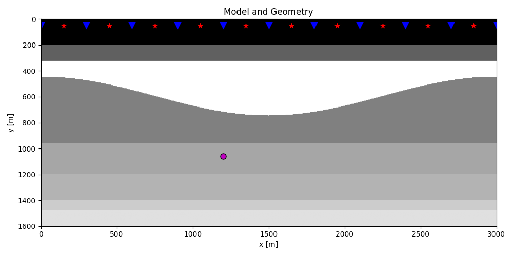
Let’s start by defining some input parameters and loading the geometry

# Input parameters
inputfile = '../testdata/marchenko/input.npz'

vel = 2400.0         # velocity
toff = 0.045         # direct arrival time shift
nsmooth = 10         # time window smoothing
nfmax = 400          # max frequency for MDC (#samples)
niter = 10           # iterations

inputdata = np.load(inputfile)

# Receivers
r = inputdata['r']
nr = r.shape[1]
dr = r[0, 1]-r[0, 0]

# Sources
s = inputdata['s']
ns = s.shape[1]
ds = s[0, 1]-s[0, 0]

# Virtual points
vs = inputdata['vs']

# Density model
rho = inputdata['rho']
z, x = inputdata['z'], inputdata['x']

plt.figure(figsize=(10, 5))
plt.imshow(rho, cmap='gray', extent=(x[0], x[-1], z[-1], z[0]))
plt.scatter(s[0, 5::10], s[1, 5::10], marker='*', s=150, c='r', edgecolors='k')
plt.scatter(r[0, ::10], r[1, ::10], marker='v', s=150, c='b', edgecolors='k')
plt.scatter(vs[0], vs[1], marker='.', s=250, c='m', edgecolors='k')
plt.axis('tight')
plt.xlabel('x [m]')
plt.ylabel('y [m]')
plt.title('Model and Geometry')
plt.xlim(x[0], x[-1])
plt.tight_layout()

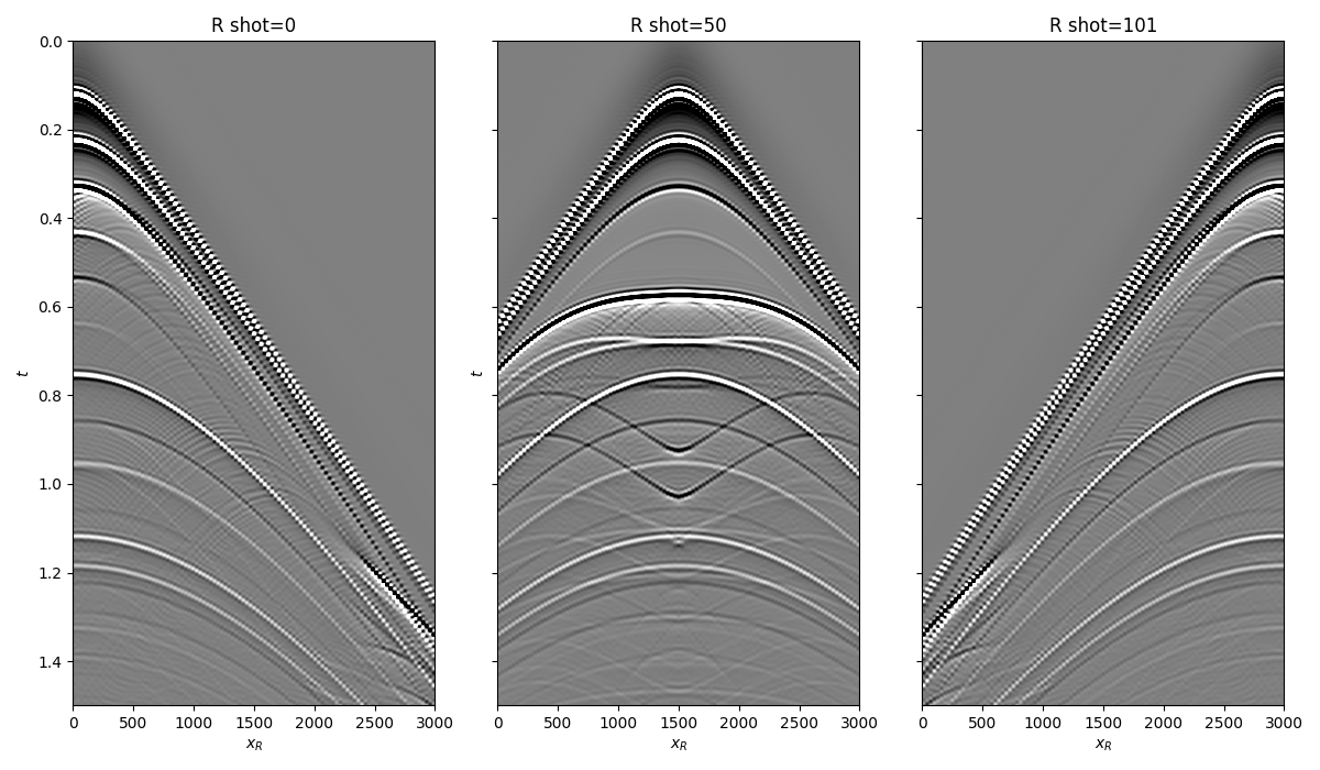
Let’s now load and display the reflection response

# Time axis
t = inputdata['t'][:-100]
ot, dt, nt = t[0], t[1]-t[0], len(t)

# Reflection data (R[s, r, t]) and subsurface fields
R = inputdata['R'][:, :, :-100]
R = np.swapaxes(R, 0, 1) # just because of how the data was saved

fig, axs = plt.subplots(1, 3, sharey=True, figsize=(12, 7))
axs[0].imshow(R[0].T, cmap='gray', vmin=-1e-2, vmax=1e-2,
              extent=(r[0, 0], r[0, -1], t[-1], t[0]))
axs[0].set_title('R shot=0')
axs[0].set_xlabel(r'$x_R$')
axs[0].set_ylabel(r'$t$')
axs[0].axis('tight')
axs[0].set_ylim(1.5, 0)
axs[1].imshow(R[ns//2].T, cmap='gray', vmin=-1e-2, vmax=1e-2,
              extent=(r[0, 0], r[0, -1], t[-1], t[0]))
axs[1].set_title('R shot=%d' %(ns//2))
axs[1].set_xlabel(r'$x_R$')
axs[1].set_ylabel(r'$t$')
axs[1].axis('tight')
axs[1].set_ylim(1.5, 0)
axs[2].imshow(R[-1].T, cmap='gray', vmin=-1e-2, vmax=1e-2,
              extent=(r[0, 0], r[0, -1], t[-1], t[0]))
axs[2].set_title('R shot=%d' %ns)
axs[2].set_xlabel(r'$x_R$')
axs[2].axis('tight')
axs[2].set_ylim(1.5, 0)
fig.tight_layout()

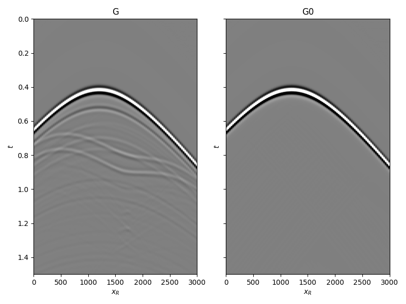
and the true and background subsurface fields

# Subsurface fields
Gsub = inputdata['Gsub'][:-100]
G0sub = inputdata['G0sub'][:-100]
wav = inputdata['wav']
wav_c = np.argmax(wav)

Gsub = np.apply_along_axis(convolve, 0, Gsub, wav, mode='full')
Gsub = Gsub[wav_c:][:nt]
G0sub = np.apply_along_axis(convolve, 0, G0sub, wav, mode='full')
G0sub = G0sub[wav_c:][:nt]

fig, axs = plt.subplots(1, 2, sharey=True, figsize=(8, 6))
axs[0].imshow(Gsub, cmap='gray', vmin=-1e6, vmax=1e6,
              extent=(r[0, 0], r[0, -1], t[-1], t[0]))
axs[0].set_title('G')
axs[0].set_xlabel(r'$x_R$')
axs[0].set_ylabel(r'$t$')
axs[0].axis('tight')
axs[0].set_ylim(1.5, 0)
axs[1].imshow(G0sub, cmap='gray', vmin=-1e6, vmax=1e6,
              extent=(r[0, 0], r[0, -1], t[-1], t[0]))
axs[1].set_title('G0')
axs[1].set_xlabel(r'$x_R$')
axs[1].set_ylabel(r'$t$')
axs[1].axis('tight')
axs[1].set_ylim(1.5, 0)
fig.tight_layout()

Let’s now create an object of the pymarchenko.neumarchenko.NeumannMarchenko class and apply redatuming for a single subsurface point vs.

# Direct arrival traveltime
trav = np.sqrt((vs[0]-r[0])**2+(vs[1]-r[1])**2)/vel

MarchenkoWM = NeumannMarchenko(R, dt=dt, dr=dr, nfmax=nfmax, wav=wav,
                               toff=toff, nsmooth=nsmooth)

f1_inv_minus, f1_inv_plus, p0_minus, g_inv_minus, g_inv_plus = \
    MarchenkoWM.apply_onepoint(trav, G0=G0sub.T, rtm=True,
                               greens=True, n_iter=niter)
g_inv_tot = g_inv_minus + g_inv_plus

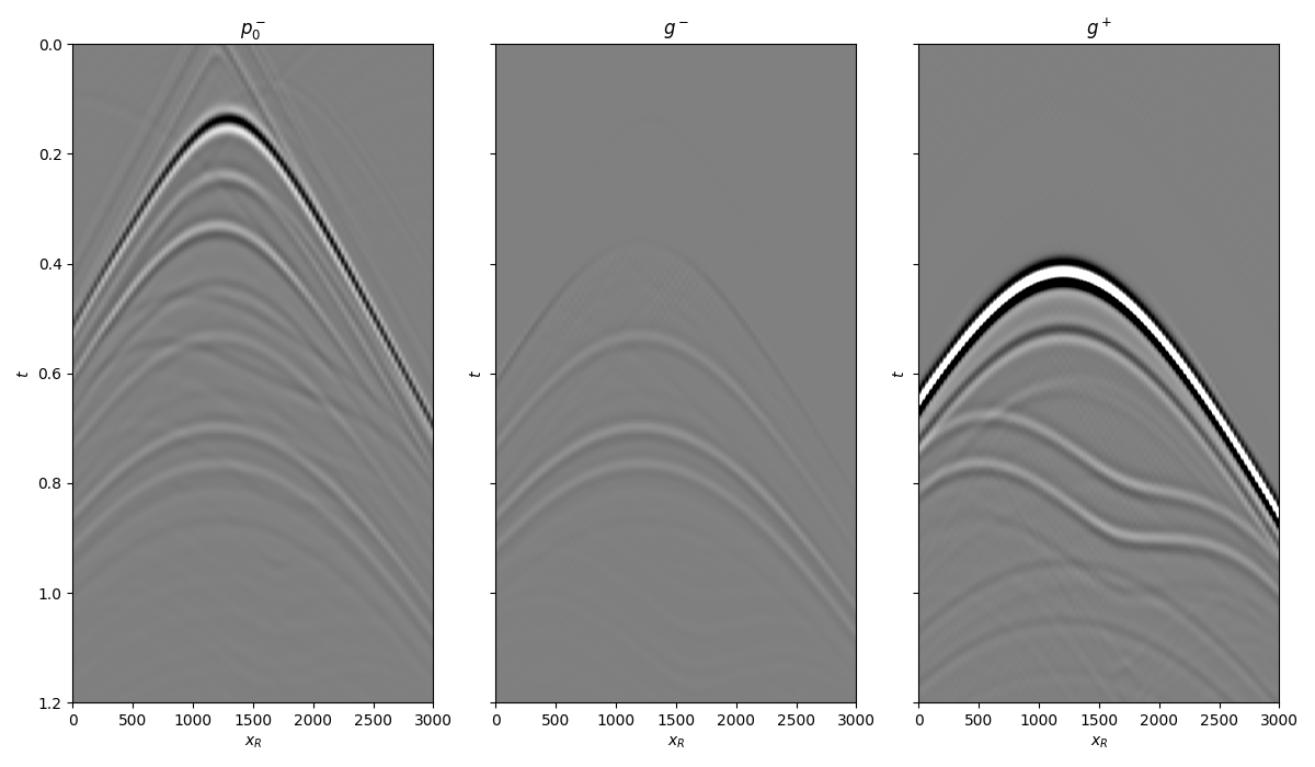
We can now compare the result of Marchenko redatuming with standard redatuming

fig, axs = plt.subplots(1, 3, sharey=True, figsize=(12, 7))
axs[0].imshow(p0_minus.T, cmap='gray', vmin=-5e5, vmax=5e5,
              extent=(r[0, 0], r[0, -1], t[-1], -t[-1]))
axs[0].set_title(r'$p_0^-$')
axs[0].set_xlabel(r'$x_R$')
axs[0].set_ylabel(r'$t$')
axs[0].axis('tight')
axs[0].set_ylim(1.2, 0)
axs[1].imshow(g_inv_minus.T, cmap='gray', vmin=-5e5, vmax=5e5,
              extent=(r[0, 0], r[0, -1], t[-1], -t[-1]))
axs[1].set_title(r'$g^-$')
axs[1].set_xlabel(r'$x_R$')
axs[1].set_ylabel(r'$t$')
axs[1].axis('tight')
axs[1].set_ylim(1.2, 0)
axs[2].imshow(g_inv_plus.T, cmap='gray', vmin=-5e5, vmax=5e5,
              extent=(r[0, 0], r[0, -1], t[-1], -t[-1]))
axs[2].set_title(r'$g^+$')
axs[2].set_xlabel(r'$x_R$')
axs[2].set_ylabel(r'$t$')
axs[2].axis('tight')
axs[2].set_ylim(1.2, 0)
fig.tight_layout()

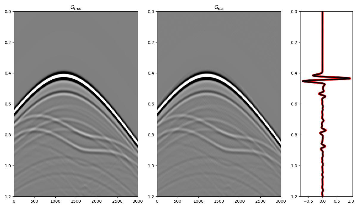
and compare the total Green’s function with the directly modelled one

fig = plt.figure(figsize=(12, 7))
ax1 = plt.subplot2grid((1, 5), (0, 0), colspan=2)
ax2 = plt.subplot2grid((1, 5), (0, 2), colspan=2)
ax3 = plt.subplot2grid((1, 5), (0, 4))
ax1.imshow(Gsub, cmap='gray', vmin=-5e5, vmax=5e5,
           extent=(r[0, 0], r[0, -1], t[-1], t[0]))
ax1.set_title(r'$G_{true}$')
axs[0].set_xlabel(r'$x_R$')
axs[0].set_ylabel(r'$t$')
ax1.axis('tight')
ax1.set_ylim(1.2, 0)
ax2.imshow(g_inv_tot.T, cmap='gray', vmin=-5e5, vmax=5e5,
           extent=(r[0, 0], r[0, -1], t[-1], -t[-1]))
ax2.set_title(r'$G_{est}$')
axs[1].set_xlabel(r'$x_R$')
axs[1].set_ylabel(r'$t$')
ax2.axis('tight')
ax2.set_ylim(1.2, 0)
ax3.plot(Gsub[:, nr//2]/Gsub.max(), t, 'r', lw=5)
ax3.plot(g_inv_tot[nr//2, nt-1:]/g_inv_tot.max(), t, 'k', lw=3)
ax3.set_ylim(1.2, 0)
fig.tight_layout()